Vertical farming lives or dies on energy economics, because lighting is usually the largest single operating cost. The whole business case reduces to two ratios: how many photons each joule buys (efficacy, µmol/J), and how much saleable yield each photon produces (a function of crop, recipe and environment). This article gives a framework to compare options on those ratios instead of on fixture price.
Efficacy is the first lever
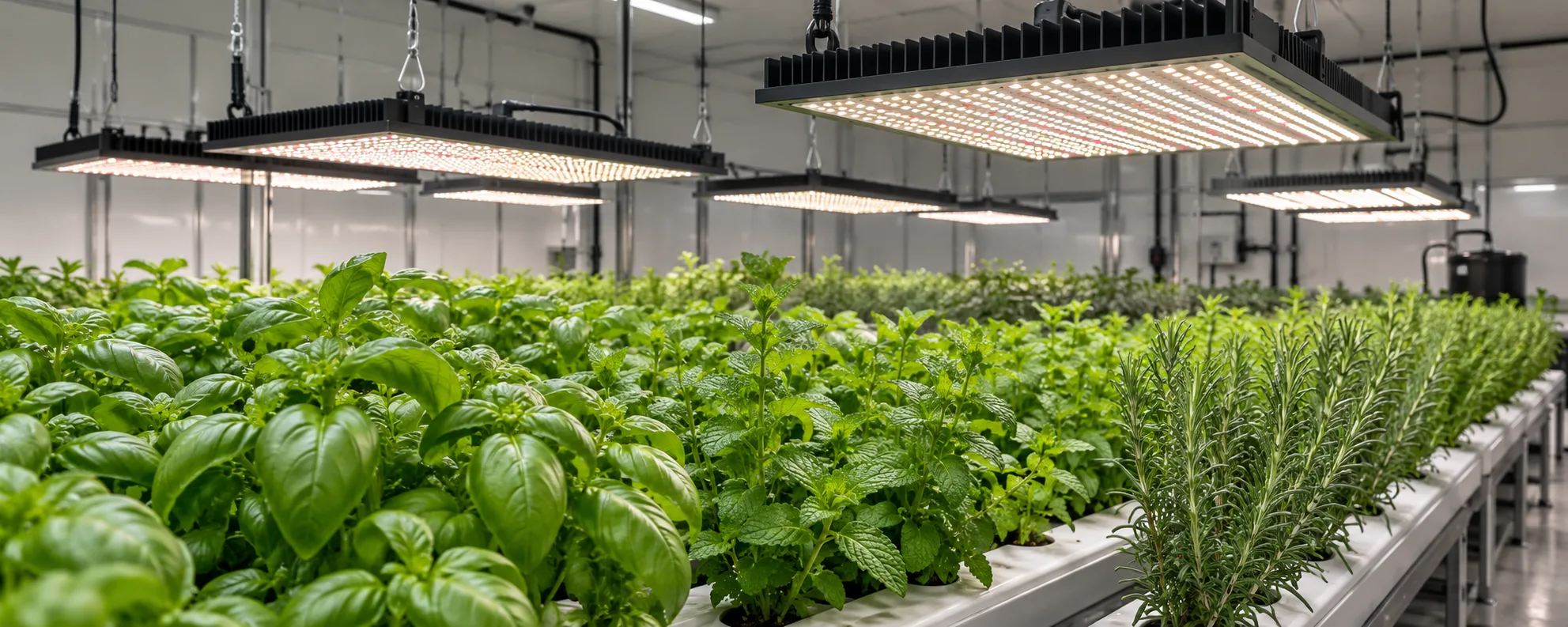
Efficacy (PPF per watt) is the most direct energy lever. A fixture at 2.4 µmol/J delivers more light per kilowatt-hour than one at 2.0, and over thousands of operating hours that gap is a large part of the electricity bill. Always ask for efficacy measured at the drive current the fixture will actually run, not a best-case number.
| Efficacy | Power for 1,000 µmol/s | Relative energy |
|---|---|---|
| 2.0 µmol/J | 500 W | 100% (baseline) |
| 2.4 µmol/J | 417 W | 83% |
| 2.8 µmol/J | 357 W | 71% |
Density and yield per photon
More tiers deliver more canopy per floor metre, but only if the crop, recipe and environment convert that light to saleable yield. Chasing density without agronomy just spreads the same photons thinner. The honest question is yield per photon at your target DLI, not raw tier count.
Cheap fixtures can be expensive
A low-efficacy fixture with a low price often costs more over five years than a higher-efficacy fixture, because lighting runs continuously. Compare lifetime energy, not sticker price.
Worked energy estimate
Ten tiers, each 1000 µmol/s required, fixture at 2.4 µmol/J: power per tier = 1000 / 2.4 = 417 W. For 10 tiers and 18 daily photoperiod hours over a 30-day month: 417 W × 10 × 18 h × 30 = 2,251,800 Wh ≈ 2,252 kWh/month for lighting. Swapping to 2.0 µmol/J raises that to 2,700 kWh — a 20 percent energy difference for the same light.
| Efficacy | Power/tier | Monthly kWh |
|---|---|---|
| 2.0 µmol/J | 500 W | 2,700 kWh |
| 2.4 µmol/J | 417 W | 2,252 kWh |
| 2.8 µmol/J | 357 W | 1,929 kWh |
Worked example: the energy cost of one kilogram of greens
This is an illustrative model, not a benchmark for any specific facility. Assume a rack producing lettuce at 220 umol/m2/s for 18 hours, fixtures at 2.6 umol/J, electricity at 0.12 per kWh, and a facility-level electricity overhead (HVAC and other loads) of 60 percent on top of fixture energy. A 3.6 m2 layer draws about 369 W of fixture power as calculated in the layout article.
- Fixture energy per layer per day: 369 W x 18 h = 6.64 kWh.
- With facility overhead at 1.6: total electrical energy = 10.6 kWh per layer per day.
- Energy cost per layer per day: 10.6 x 0.12 = about 1.27 per day.
- If that layer yields 2.5 kg of saleable lettuce per cycle of 28 days, layer output per day is about 0.089 kg.
- Energy cost per kg: 1.27 / 0.089 = roughly 14.3 per kg attributed to total facility electricity.
- Fixture-only share: 6.64 x 0.12 / 0.089 = about 8.9 per kg; the rest is climate control and other loads.
Every assumption in this model moves the answer: yield per layer, cycle time, electricity price and the overhead factor are all site specific. The value of the exercise is the structure, because it shows which lever matters. Doubling efficacy from 2.0 to 2.6 umol/J cuts fixture energy by about 23 percent; improving yield per layer by 20 percent cuts energy per kg by 17 percent with the same fixtures. Operations usually find yield and cycle time levers bigger than fixture levers, which is why the model must include them.
Where the money actually goes
Fixed versus variable costs
Lighting is partly a fixed decision (capex plus a long depreciation tail) and partly a variable one (electricity and maintenance). The variable part is manageable in real time: dimming decisions, photoperiod length, crop scheduling to keep racks full and demand-charge management. The fixed part is locked at purchase: efficacy, spectrum, build quality and warranty terms determine maintenance cost for years. This is why procurement scrutiny at purchase time pays off for the life of the installation.
A simple payback checklist
- Record measured (not estimated) energy per kg for at least one full crop cycle before and after any lighting change.
- Track yield per layer, cycle time and unsaleable percentage together, because a lighting change that raises one and damages another can net zero.
- Include controls capability in the capex comparison; a fixture that cannot dim to shoulder-month levels wastes its own efficiency.
- Ask suppliers for L90 lifetime at your room temperature, not just a headline hour figure at ideal conditions.
- Price the spares kit and driver replacement cost at year 5 into the comparison, not just the fixture price.
Common mistakes in vertical farming lighting economics
Economic models fail before the farm does. These are the modelling errors that distort lighting decisions:
- Counting fixture energy and ignoring the climate load the fixtures create; at high intensity the HVAC share is not optional arithmetic.
- Using nameplate efficacy instead of efficacy at the actual operating point (dimmed, warm, dirty).
- Modelling yield per layer from the best tier and applying it to all tiers; bottom tiers underperform top tiers in every real building.
- Amortising capex over a lifetime the warranty does not support, then discovering driver replacement economics at year five.
- Excluding controls from the comparison because they look like overhead; un-dimmed shoulder periods quietly destroy the efficiency advantage.
- Ignoring demand charges and tariff windows, which can move the effective electricity price more than a fixture upgrade moves the efficacy.
Sensitivity: which variable deserves the next investment
Running the tornado
A sensitivity pass takes one afternoon: vary each input by 10 percent and record the effect on cost per kilogram. In most models the order comes out roughly like this: yield per layer, cycle time, electricity price, facility overhead factor, fixture efficacy, fixture price. The value is directional, not exact; it tells you that a 10 percent improvement in cycle time usually outweighs a 10 percent improvement in efficacy, which is why a controls upgrade can beat a fixture upgrade on payback even though the fixture is the more visible purchase.
The measurement that anchors the model
Every model above rests on one measured anchor: energy and output for one real layer over one real cycle. Facility-level averages blur the tiers together; the layer-level measurement (kWh in, saleable grams out, days elapsed) is what makes the model yours rather than a consultants template. Once the anchor exists, every proposal (new spectrum, longer photoperiod, denser tray) can be priced against the same baseline instead of argued in the abstract.
| Input changed by 10 percent | Direction | Approx. effect on energy cost per kg |
|---|---|---|
| Yield per layer | Increase | About -9 percent |
| Cycle time | Decrease | About -8 percent |
| Electricity price | Increase | About +10 percent |
| Fixture efficacy | Increase | About -2 to -3 percent |
| Fixture purchase price | Decrease | Small effect on opex per kg |
Reading a supplier quote the economic way
Quotes arrive formatted for comparison on price per fixture, which is almost the least informative number on the page. The economic way to read one:
- Normalize to cost per delivered PPF at canopy level: fixture price plus mounting, wiring and controls, divided by the PPF the layout actually delivers.
- Convert efficacy into annual energy cost at your tariff and photoperiod, per fixture; a 0.2 umol/J difference is a small number per fixture and a large one across a facility.
- Price the warranty economics: length, what invalidates it, and the cost of a driver replacement event at year 5.
- Check dimming range against your operating profile; a fixture that cannot reach shoulder-month outputs delivers efficiency you will never use.
- Ask for the L90 lifetime at your room temperature, then compare depreciation assumptions across quotes on equal terms.
- Include the spares kit and its price, because the first driver failure should not become an emergency purchase.
Two quotes can differ by 15 percent on price per fixture and still reverse their order on cost per delivered PPF over five years. Running this comparison takes an hour and routinely changes the purchase decision; it is the highest-paid hour in the procurement process.
References you can verify
- e-GRO - lighting economics and controlled environment notes
- Controlled Environment Agriculture Center, University of Arizona
- DesignLights Consortium - horticultural lighting qualified products and efficacy data
Frequently asked questions
Is efficacy the only energy lever?+
No — photoperiod, DLI target, density and cooling all matter. But efficacy is the cleanest, fixture-level lever and the first thing to compare.
Should I maximise tiers?+
Only if yield per photon holds. More tiers spread light and air; if agronomy does not keep up, you gain canopy but not saleable yield.
How do I compare fixtures fairly?+
Compare efficacy at real drive current, warranty, thermal design and uniformity — not sticker price alone.
Does cooling energy count?+
Yes. In dense vertical farms the light’s heat loads HVAC; lower radiant-heat fixtures can cut cooling cost too.
What is the single best metric?+
Yield per photon at your target DLI, because it captures both the light you buy and what it returns. Efficacy is the input side of that.
Are these energy numbers guaranteed?+
No. They are estimates from stated assumptions (efficacy, hours, tiers). Your real bill depends on your recipe, climate and tariffs.
Modelling vertical-farm economics?
Share tiers, target DLI and tariff. We model lighting energy and compare efficacy options.
Get a Grow Light Solution